Overview of Heat Exchanger Models¶

This tutorial shows an overview of the different heat exchanger models available in TESPy. The table below indicates the different types and how they compare in general. Further down we have created a problem which models the heat exchanger with a variety of the mentioned types and we show the differences in the results.

Overview table¶

type		speed	accuracy*	internal pinch
SimpleHeatExchanger	0D	fastest	lowest	no
HeatExchanger	0D	very fast	lower	no
ParallelFlowHeatExchanger	0D	very fast	lower	no
Desuperheater	0D	very fast	lower	no
Condenser	0D	very fast	low	(no)
MovingBoundaryHeatExchanger	1D	mid	high	yes
SectionedHeatExchanger	1D	slow	highest	yes

Note

The accuracy depends on the context. In many contexts, the standard 0D heat exchanger components can be just as accurate as the 1D models.
The calculation speed also depends on context for the SectionedHeatExchanger:
1. The number of specified sections influences the speed.
2. If you impose td_pinch or UA to your model it will be significantly slower compared to other models, especially with a high number of sections.
3. If you do not specify td_pinch or UA the sectioning is only applied once in the postprocessing; this takes more time than other heat exchanger types but is still relatively fast.

import pandas as pd
import matplotlib.patches as mpatches
from matplotlib import pyplot as plt
from tespy.components import (
    Condenser,
    HeatExchanger,
    MovingBoundaryHeatExchanger,
    SectionedHeatExchanger,
    Sink,
    Source,
)
from tespy.connections import Connection
from tespy.networks import Network
from tespy.tools.fluid_properties import h_mix_pQ

annotation_color = "black"
results = []


def make_network(heatex):

    nw = Network()
    nw.units.set_defaults(
        temperature="°C",
        pressure="bar",
        pressure_difference="bar",
        heat="MW",
        heat_transfer_coefficient="kW/K"
    )
    so1 = Source("source 1")
    so2 = Source("source 2")
    si1 = Sink("sink 1")
    si2 = Sink("sink 2")
    c1 = Connection(so1, "out1", heatex, "in1", label="c1")
    c2 = Connection(heatex, "out1", si1, "in1", label="c2")
    d1 = Connection(so2, "out1", heatex, "in2", label="d1")
    d2 = Connection(heatex, "out2", si2, "in1", label="d2")
    nw.add_conns(c1, c2, d1, d2)
    c1.set_attr(fluid={"R290": 1}, td_dew=50, T_dew=60, m=5)
    c2.set_attr(td_bubble=5)
    d1.set_attr(fluid={"water": 1}, p=1, T=45)
    d2.set_attr(T=55)
    heatex.set_attr(dp1=0, dp2=0)
    return nw, c1, c2, d1, d2

Matplotlib is building the font cache; this may take a moment.

Model comparisons¶

For the model comparison we have selected a typical problem: the condensation of a working fluid in a heat pump to heat up water. The boundary conditions are listed in the table below.

label	Specification	value	unit
c1	fluid	R290	-
	mass flow	5	kg/s
	dew line temperature	60	°C
	superheating	50	°C
c2	subcooling	5	°C
d1	fluid	water	-
	temperature	45	°C
	pressure	1	bar
d2	temperature	55	°C
heatexchanger	pressure drops	0	bar

Attention

Keep in mind: under different boundary conditions (e.g. no phase change) results of this comparison may vary a lot. There might be conditions where the 0D components yield very similar results, or where the deviation is even higher.

For the calculation of the results the following equations apply:

\[ \begin{align}\begin{aligned}\begin{split}\Delta \theta_\text{log} = \frac{\Delta T_{i} - \Delta T_{i+1}}{\ln \frac{\Delta T_{i}}{\Delta T_{i+1}}}\\\end{split}\\\begin{split}kA=\frac{\dot Q}{\Delta \theta_\text{log}}\\\end{split}\\\begin{split}UA_{i}=\frac{\dot Q_{i}}{\Delta \theta_{\text{log,}i}}\\\end{split}\\UA=\sum UA_{i} \end{aligned}\end{align} \]

For the calculation of \(kA\) the terminal temperature differences ttd_u and ttd_l are considered as \(\Delta T_0\) and \(\Delta T_1\). For the calculation of \(UA\), the internal temperature differences \(\Delta T_{i}\) in each section of the heat exchanger are employed.

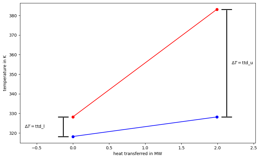
HeatExchanger¶

hx_0d = HeatExchanger("heatexchanger")
nw, c1, c2, d1, d2 = make_network(hx_0d)
nw.solve("design")

results.append({
    "model": "HeatExchanger",
    "minimum pinch (K)": f"n/a ({hx_0d.ttd_min.val:.1f})",
    "kA (kW/K)": f"{hx_0d.kA.val:.1f}",
    "UA (kW/K)": "n/a",
})

heat = [0, abs(hx_0d.Q.val)]
T_hot = [c2.T.val_SI, c1.T.val_SI]
T_cold = [d1.T.val_SI, d2.T.val_SI]

fig, ax = plt.subplots(1, figsize=(10, 6))

ax.plot(heat, T_hot, "o-", color="red")
ax.plot(heat, T_cold, "o-", color="blue")

offset = heat[-1] / 15
bar_len = heat[-1] / 15

bracket = mpatches.FancyArrowPatch(
    (heat[-1] * (1 + 1 / 15), T_cold[-1]), (heat[-1] * (1 + 1 / 15), T_hot[-1]),
    connectionstyle="bar,angle=0,fraction=0", arrowstyle="-", linewidth=2, color=annotation_color,
)
ax.add_patch(bracket)
ax.plot([heat[-1] + offset - bar_len/2, heat[-1] + offset + bar_len/2], [T_hot[-1], T_hot[-1]], color=annotation_color, lw=2)
ax.plot([heat[-1] + offset - bar_len/2, heat[-1] + offset + bar_len/2], [T_cold[-1], T_cold[-1]], color=annotation_color, lw=2)
ax.text(heat[-1] * 1.1, (T_hot[-1] + T_cold[-1]) / 2, r"$\Delta T = \text{ttd\_u}$", va="center", color=annotation_color)

bracket = mpatches.FancyArrowPatch(
    (0 - offset, T_cold[0]), (0 - offset, T_hot[0]),
    connectionstyle="bar,angle=0,fraction=0", arrowstyle="-", linewidth=2, color=annotation_color,
)
ax.add_patch(bracket)
ax.text(heat[0] - offset * 5, (T_hot[0] + T_cold[0]) / 2, r"$\Delta T = \text{ttd\_l}$", va="center", color=annotation_color)
ax.plot([heat[0] - offset - bar_len/2, heat[0] - offset + bar_len/2], [T_hot[0], T_hot[0]], color=annotation_color, lw=2)
ax.plot([heat[0] - offset - bar_len/2, heat[0] - offset + bar_len/2], [T_cold[0], T_cold[0]], color=annotation_color, lw=2)

ax.set_xbound([-5.5 * offset, heat[-1] + 4 * offset])
ax.set_ylabel("temperature in K")
ax.set_xlabel("heat transferred in MW")
plt.show()

RuntimeWarning: invalid value encountered in scalar divide

 iter  | residual   | progress   | massflow   | pressure   | enthalpy   | fluid      | component  
-------+------------+------------+------------+------------+------------+------------+------------
 1     | 1.93e+06   | 0 %        | 4.61e+01   | 0.00e+00   | 0.00e+00   | 0.00e+00   | 0.00e+00   
 2     | 4.87e-06   | 100 %      | 1.17e-10   | 0.00e+00   | 0.00e+00   | 0.00e+00   | 0.00e+00   
 3     | 0.00e+00   | 100 %      | 0.00e+00   | 0.00e+00   | 0.00e+00   | 0.00e+00   | 0.00e+00   
 4     | 2.33e-10   | 100 %      | 5.57e-15   | 0.00e+00   | 0.00e+00   | 0.00e+00   | 0.00e+00   
Total iterations: 4, Calculation time: 0.00 s, Iterations per second: 1851.99

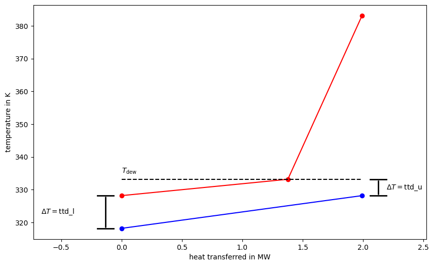
../_images/f9e43bfd26cd843ea93477b5e0e978f656b5255d95f1759176bb37c4705c79fa.png

Condenser¶

In the condenser the upper terminal temperature difference is assigned to the temperature difference between the dew line temperature of the condensing fluid and the outlet temperature of the cold fluid.

hx_cond = Condenser("heatexchanger")
nw, c1, c2, d1, d2 = make_network(hx_cond)
hx_cond.set_attr(subcooling=True)
nw.solve("design")

results.append({
    "model": "Condenser",
    "minimum pinch (K)": f"n/a ({hx_cond.ttd_min.val:.1f})",
    "kA (kW/K)": f"{hx_cond.kA.val:.1f}",
    "UA (kW/K)": "n/a",
})

T_cond = c2.T.val_SI - c2.calc_td_dew()
heat_to_cond = c1.m.val_SI * (h_mix_pQ(c2.p.val_SI, 1, c2.fluid_data) - c2.h.val_SI) / 1e6
heat = [0, heat_to_cond, abs(hx_cond.Q.val)]
T_hot = [c2.T.val_SI, T_cond, c1.T.val_SI]
T_cold = [d1.T.val_SI, d2.T.val_SI]

fig, ax = plt.subplots(1, figsize=(10, 6))
ax.plot(heat, T_hot, "o-", color="red")
ax.plot([heat[0], heat[-1]], [T_cold[0], T_cold[-1]], "o-", color="blue")
ax.plot([heat[0], heat[-1]], [T_cond, T_cond], "--", color=annotation_color)
ax.text(heat[0], T_cond + 2.5, r"$T_\text{dew}$", va="center", color=annotation_color)

offset = heat[-1] / 15
bar_len = heat[-1] / 15

bracket = mpatches.FancyArrowPatch(
    (heat[-1] * (1 + 1 / 15), T_cold[-1]), (heat[-1] * (1 + 1 / 15), T_cond),
    connectionstyle="bar,angle=0,fraction=0", arrowstyle="-", linewidth=2, color=annotation_color,
)
ax.add_patch(bracket)
ax.plot([heat[-1] + offset - bar_len/2, heat[-1] + offset + bar_len/2], [T_cond, T_cond], color=annotation_color, lw=2)
ax.plot([heat[-1] + offset - bar_len/2, heat[-1] + offset + bar_len/2], [T_cold[-1], T_cold[-1]], color=annotation_color, lw=2)
ax.text(heat[-1] * 1.1, (T_cond + T_cold[-1]) / 2, r"$\Delta T = \text{ttd\_u}$", va="center", color=annotation_color)

bracket = mpatches.FancyArrowPatch(
    (0 - offset, T_cold[0]), (0 - offset, T_hot[0]),
    connectionstyle="bar,angle=0,fraction=0", arrowstyle="-", linewidth=2, color=annotation_color,
)
ax.add_patch(bracket)
ax.text(heat[0] - offset * 5, (T_hot[0] + T_cold[0]) / 2, r"$\Delta T = \text{ttd\_l}$", va="center", color=annotation_color)
ax.plot([heat[0] - offset - bar_len/2, heat[0] - offset + bar_len/2], [T_hot[0], T_hot[0]], color=annotation_color, lw=2)
ax.plot([heat[0] - offset - bar_len/2, heat[0] - offset + bar_len/2], [T_cold[0], T_cold[0]], color=annotation_color, lw=2)

ax.set_xbound([-5.5 * offset, heat[-1] + 4 * offset])
ax.set_ylabel("temperature in K")
ax.set_xlabel("heat transferred in MW")
plt.show()

RuntimeWarning: invalid value encountered in scalar divide

 iter  | residual   | progress   | massflow   | pressure   | enthalpy   | fluid      | component  
-------+------------+------------+------------+------------+------------+------------+------------
 1     | 1.93e+06   | 0 %        | 4.61e+01   | 0.00e+00   | 0.00e+00   | 0.00e+00   | 0.00e+00   
 2     | 4.87e-06   | 100 %      | 1.17e-10   | 0.00e+00   | 0.00e+00   | 0.00e+00   | 0.00e+00   
 3     | 0.00e+00   | 100 %      | 0.00e+00   | 0.00e+00   | 0.00e+00   | 0.00e+00   | 0.00e+00   
 4     | 2.33e-10   | 100 %      | 5.57e-15   | 0.00e+00   | 0.00e+00   | 0.00e+00   | 0.00e+00   
Total iterations: 4, Calculation time: 0.00 s, Iterations per second: 2078.45

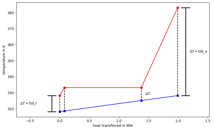
../_images/f7d66fc15ee54d8e4068774281c4ee09128d991117d1c5690a3caebf39367f16.png

MovingBoundaryHeatExchanger¶

The moving boundary model sections the heat exchange into three different sections at the phase change points.

hx_mb = MovingBoundaryHeatExchanger("heatexchanger")
nw, c1, c2, d1, d2 = make_network(hx_mb)
nw.solve("design")

heat, T_hot, T_cold, _, _ = hx_mb.calc_sections()
heat /= 1e6

results.append({
    "model": "MovingBoundaryHeatExchanger",
    "minimum pinch (K)": f"{hx_mb.td_pinch.val:.2f}",
    "kA (kW/K)": f"{hx_mb.kA.val:.1f}",
    "UA (kW/K)": f"{hx_mb.UA.val:.1f}",
})

fig, ax = plt.subplots(1, figsize=(10, 6))
ax.plot((heat, heat), (list(T_hot), list(T_cold)), color=annotation_color, linestyle="--")
ax.text(heat[2] * 1.05, (T_hot[2] + T_cold[2]) / 2, r"$\Delta T_\text{i}$", va="center", color=annotation_color)
ax.plot(heat, T_hot, "o-", color="red")
ax.plot(heat, T_cold, "o-", color="blue")

offset = heat[-1] / 15
bar_len = heat[-1] / 15

bracket = mpatches.FancyArrowPatch(
    (heat[-1] * (1 + 1 / 15), T_cold[-1]), (heat[-1] * (1 + 1 / 15), T_hot[-1]),
    connectionstyle="bar,angle=0,fraction=0", arrowstyle="-", linewidth=2, color=annotation_color,
)
ax.add_patch(bracket)
ax.plot([heat[-1] + offset - bar_len/2, heat[-1] + offset + bar_len/2], [T_hot[-1], T_hot[-1]], color=annotation_color, lw=2)
ax.plot([heat[-1] + offset - bar_len/2, heat[-1] + offset + bar_len/2], [T_cold[-1], T_cold[-1]], color=annotation_color, lw=2)
ax.text(heat[-1] * 1.1, (T_hot[-1] + T_cold[-1]) / 2, r"$\Delta T = \text{ttd\_u}$", va="center", color=annotation_color)

bracket = mpatches.FancyArrowPatch(
    (0 - offset, T_cold[0]), (0 - offset, T_hot[0]),
    connectionstyle="bar,angle=0,fraction=0", arrowstyle="-", linewidth=2, color=annotation_color,
)
ax.add_patch(bracket)
ax.text(heat[0] - offset * 5, (T_hot[0] + T_cold[0]) / 2, r"$\Delta T = \text{ttd\_l}$", va="center", color=annotation_color)
ax.plot([heat[0] - offset - bar_len/2, heat[0] - offset + bar_len/2], [T_hot[0], T_hot[0]], color=annotation_color, lw=2)
ax.plot([heat[0] - offset - bar_len/2, heat[0] - offset + bar_len/2], [T_cold[0], T_cold[0]], color=annotation_color, lw=2)

ax.set_xbound([-5.5 * offset, heat[-1] + 4 * offset])
ax.set_ylabel("temperature in K")
ax.set_xlabel("heat transferred in MW")
plt.show()

 iter  | residual   | progress   | massflow   | pressure   | enthalpy   | fluid      | component  
-------+------------+------------+------------+------------+------------+------------+------------
 1     | 1.93e+06   | 0 %        | 4.61e+01   | 0.00e+00   | 0.00e+00   | 0.00e+00   | 0.00e+00   
 2     | 4.87e-06   | 100 %      | 1.17e-10   | 0.00e+00   | 0.00e+00   | 0.00e+00   | 0.00e+00   
 3     | 0.00e+00   | 100 %      | 0.00e+00   | 0.00e+00   | 0.00e+00   | 0.00e+00   | 0.00e+00   
 4     | 2.33e-10   | 100 %      | 5.57e-15   | 0.00e+00   | 0.00e+00   | 0.00e+00   | 0.00e+00   
Total iterations: 4, Calculation time: 0.00 s, Iterations per second: 2149.27

RuntimeWarning: invalid value encountered in scalar divide

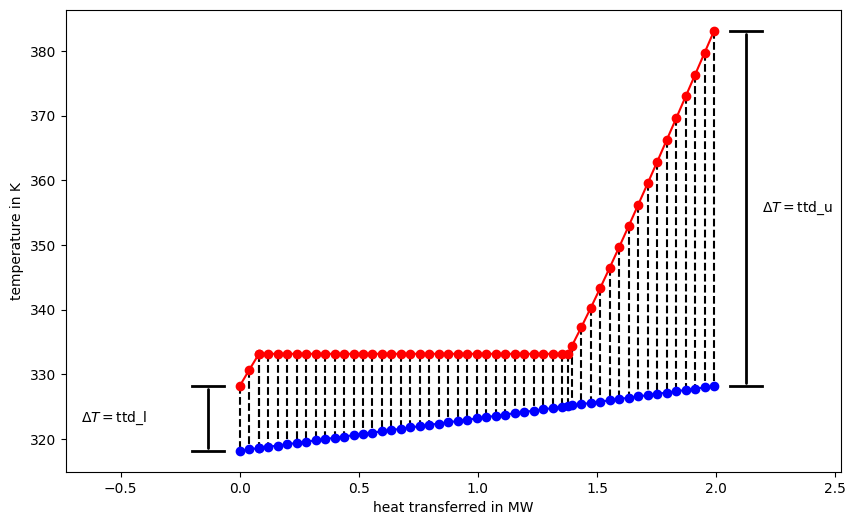
../_images/b583cf753572b20ce40f830179c9cefdbb5f620732a701e420b738d236d37cda.png

SectionedHeatExchanger¶

The sectioned model sections the heat exchange into 50 sections by default and extra sections are inserted at the moving boundaries (note the smaller sections in between).

hx_sectioned = SectionedHeatExchanger("heatexchanger")
nw_sectioned, c1, c2, d1, d2 = make_network(hx_sectioned)
nw_sectioned.solve("design")

heat_50secs, T_hot_50secs, T_cold_50secs, _, _ = hx_sectioned.calc_sections()
heat_50secs /= 1e6

results.append({
    "model": "SectionedHeatExchanger (50 sections)",
    "minimum pinch (K)": f"{hx_sectioned.td_pinch.val:.2f}",
    "kA (kW/K)": f"{hx_sectioned.kA.val:.1f}",
    "UA (kW/K)": f"{hx_sectioned.UA.val:.1f}",
})

fig, ax = plt.subplots(1, figsize=(10, 6))
ax.plot((heat_50secs, heat_50secs), (list(T_hot_50secs), list(T_cold_50secs)), color=annotation_color, linestyle="--")
ax.plot(heat_50secs, T_hot_50secs, "o-", color="red")
ax.plot(heat_50secs, T_cold_50secs, "o-", color="blue")

offset = heat_50secs[-1] / 15
bar_len = heat_50secs[-1] / 15

bracket = mpatches.FancyArrowPatch(
    (heat_50secs[-1] * (1 + 1 / 15), T_cold_50secs[-1]), (heat_50secs[-1] * (1 + 1 / 15), T_hot_50secs[-1]),
    connectionstyle="bar,angle=0,fraction=0", arrowstyle="-", linewidth=2, color=annotation_color,
)
ax.add_patch(bracket)
ax.plot([heat_50secs[-1] + offset - bar_len/2, heat_50secs[-1] + offset + bar_len/2], [T_hot_50secs[-1], T_hot_50secs[-1]], color=annotation_color, lw=2)
ax.plot([heat_50secs[-1] + offset - bar_len/2, heat_50secs[-1] + offset + bar_len/2], [T_cold_50secs[-1], T_cold_50secs[-1]], color=annotation_color, lw=2)
ax.text(heat_50secs[-1] * 1.1, (T_hot_50secs[-1] + T_cold_50secs[-1]) / 2, r"$\Delta T = \text{ttd\_u}$", va="center", color=annotation_color)

bracket = mpatches.FancyArrowPatch(
    (0 - offset, T_cold_50secs[0]), (0 - offset, T_hot_50secs[0]),
    connectionstyle="bar,angle=0,fraction=0", arrowstyle="-", linewidth=2, color=annotation_color,
)
ax.add_patch(bracket)
ax.text(heat_50secs[0] - offset * 5, (T_hot_50secs[0] + T_cold_50secs[0]) / 2, r"$\Delta T = \text{ttd\_l}$", va="center", color=annotation_color)
ax.plot([heat_50secs[0] - offset - bar_len/2, heat_50secs[0] - offset + bar_len/2], [T_hot_50secs[0], T_hot_50secs[0]], color=annotation_color, lw=2)
ax.plot([heat_50secs[0] - offset - bar_len/2, heat_50secs[0] - offset + bar_len/2], [T_cold_50secs[0], T_cold_50secs[0]], color=annotation_color, lw=2)

ax.set_xbound([-5.5 * offset, heat_50secs[-1] + 4 * offset])
ax.set_ylabel("temperature in K")
ax.set_xlabel("heat transferred in MW")
plt.show()

RuntimeWarning: invalid value encountered in scalar divide

 iter  | residual   | progress   | massflow   | pressure   | enthalpy   | fluid      | component  
-------+------------+------------+------------+------------+------------+------------+------------
 1     | 1.93e+06   | 0 %        | 4.61e+01   | 0.00e+00   | 0.00e+00   | 0.00e+00   | 0.00e+00   
 2     | 4.87e-06   | 100 %      | 1.17e-10   | 0.00e+00   | 0.00e+00   | 0.00e+00   | 0.00e+00   
 3     | 0.00e+00   | 100 %      | 0.00e+00   | 0.00e+00   | 0.00e+00   | 0.00e+00   | 0.00e+00   
 4     | 2.33e-10   | 100 %      | 5.57e-15   | 0.00e+00   | 0.00e+00   | 0.00e+00   | 0.00e+00   
Total iterations: 4, Calculation time: 0.00 s, Iterations per second: 2187.67

../_images/d0362719f768da2cf95cdddcd5879ae7c1cf0de5047792c296f6a698eb50048e.png

hx_sectioned.set_attr(num_sections=6)
nw_sectioned.solve("design")
heat_6secs, T_hot_6secs, T_cold_6secs, _, _ = hx_sectioned.calc_sections()
heat_6secs /= 1e6

results.append({
    "model": "SectionedHeatExchanger (6 sections)",
    "minimum pinch (K)": f"{hx_sectioned.td_pinch.val:.2f}",
    "kA (kW/K)": f"{hx_sectioned.kA.val:.1f}",
    "UA (kW/K)": f"{hx_sectioned.UA.val:.1f}",
})

 iter  | residual   | progress   | massflow   | pressure   | enthalpy   | fluid      | component  
-------+------------+------------+------------+------------+------------+------------+------------
 1     | 0.00e+00   | 100 %      | 0.00e+00   | 0.00e+00   | 0.00e+00   | 0.00e+00   | 0.00e+00   
 2     | 2.33e-10   | 100 %      | 5.57e-15   | 0.00e+00   | 0.00e+00   | 0.00e+00   | 0.00e+00   
 3     | 0.00e+00   | 100 %      | 0.00e+00   | 0.00e+00   | 0.00e+00   | 0.00e+00   | 0.00e+00   
 4     | 0.00e+00   | 100 %      | 0.00e+00   | 0.00e+00   | 0.00e+00   | 0.00e+00   | 0.00e+00   
Total iterations: 4, Calculation time: 0.00 s, Iterations per second: 2052.26

pd.DataFrame(results).set_index("model").style

	minimum pinch (K)	kA (kW/K)	UA (kW/K)
model
HeatExchanger	n/a (10.0)	75.5	n/a
Condenser	n/a (5.0)	276.1	n/a
MovingBoundaryHeatExchanger	8.08	75.5	149.4
SectionedHeatExchanger (50 sections)	8.08	75.5	150.2
SectionedHeatExchanger (6 sections)	8.08	75.5	149.9

MovingBoundary and Sectioned models¶

Comparing these two models, we see almost identical results in the cases shown above. However, this is not necessarily the case. There are situations where these models may yield slightly different results. This is specifically the case when there is a curvature in the isobars (e.g. supercritical conditions near the critical point) or when there is a pressure drop in a pure liquid phase nearing the two-phase region.

First, we have a look at different comparisons of the two models, where the performance is very similar.

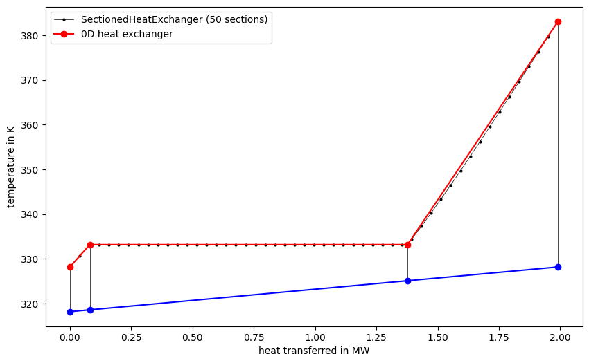
Comparing different number of sections¶

The following graph shows the comparison of a MovingBoundaryHeatExchanger and a SectionedHeatExchanger. There is a very small difference in the desuperheating section.

hx_sectioned.set_attr(num_sections=1)
nw_sectioned.solve("design")

heat_1sec, T_hot_1sec, T_cold_1sec, _, _ = hx_sectioned.calc_sections()
heat_1sec /= 1e6

fig, ax = plt.subplots(1, figsize=(10, 6))
ax.plot((heat_1sec, heat_1sec), (list(T_hot_1sec), list(T_cold_1sec)), color=annotation_color, linestyle="-", linewidth=0.5)
ax.plot(heat_50secs, T_hot_50secs, "o-", color=annotation_color, markersize=2, linewidth=0.5, label="SectionedHeatExchanger (50 sections)")
ax.plot(heat_1sec, T_hot_1sec, "o-", color="red", label="0D heat exchanger")
ax.plot(heat_1sec, T_cold_1sec, "o-", color="blue")
ax.set_ylabel("temperature in K")
ax.set_xlabel("heat transferred in MW")
ax.legend()
plt.show()

 iter  | residual   | progress   | massflow   | pressure   | enthalpy   | fluid      | component  
-------+------------+------------+------------+------------+------------+------------+------------
 1     | 0.00e+00   | 100 %      | 0.00e+00   | 0.00e+00   | 0.00e+00   | 0.00e+00   | 0.00e+00   
 2     | 2.33e-10   | 100 %      | 5.57e-15   | 0.00e+00   | 0.00e+00   | 0.00e+00   | 0.00e+00   
 3     | 0.00e+00   | 100 %      | 0.00e+00   | 0.00e+00   | 0.00e+00   | 0.00e+00   | 0.00e+00   
 4     | 0.00e+00   | 100 %      | 0.00e+00   | 0.00e+00   | 0.00e+00   | 0.00e+00   | 0.00e+00   
Total iterations: 4, Calculation time: 0.00 s, Iterations per second: 2456.40

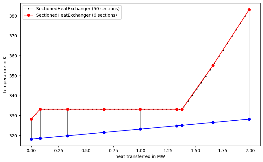
../_images/914c26143a15a857463771125ca9e3979a8fa4a9923f198dc16a5e3153fbcecf.png

And two sectioned models with different numbers of sections, where we can see that already with a few sections we can yield quite good results.

fig, ax = plt.subplots(1, figsize=(10, 6))
ax.plot((heat_6secs, heat_6secs), (list(T_hot_6secs), list(T_cold_6secs)), color=annotation_color, linestyle="-", linewidth=0.5)
ax.plot(heat_50secs, T_hot_50secs, "o-", color=annotation_color, markersize=2, linewidth=0.5, label="SectionedHeatExchanger (50 sections)")
ax.plot(heat_6secs, T_hot_6secs, "o-", color="red", label="SectionedHeatExchanger (6 sections)")
ax.plot(heat_6secs, T_cold_6secs, "o-", color="blue")
ax.set_ylabel("temperature in K")
ax.set_xlabel("heat transferred in MW")
ax.legend()
plt.show()

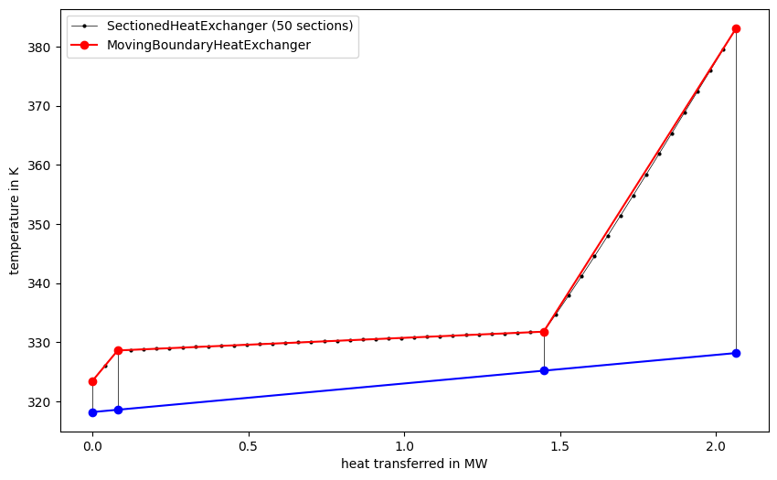
../_images/c042db8accf83241c7baf1e02f147183442a98e9a52a4a40c00e43ae8b5ab9c6.png

Considering pressure drop¶

Since both types of models can consider pressure drop (in the same way), they match quite well again.

hx_sectioned = SectionedHeatExchanger("heatexchanger")
nw_sectioned, c1, c2, d1, d2 = make_network(hx_sectioned)
hx_sectioned.set_attr(dp1=2, dp2=0.5)
nw_sectioned.solve("design")
heat_sect, T_hot_sect, T_cold_sect, _, _ = hx_sectioned.calc_sections()
heat_sect /= 1e6

hx_mb = MovingBoundaryHeatExchanger("heatexchanger")
nw_mb, c1, c2, d1, d2 = make_network(hx_mb)
hx_mb.set_attr(dp1=2, dp2=0.5)
nw_mb.solve("design")
heat_mb, T_hot_mb, T_cold_mb, _, _ = hx_mb.calc_sections()
heat_mb /= 1e6

fig, ax = plt.subplots(1, figsize=(10, 6))
ax.plot((heat_mb, heat_mb), (list(T_hot_mb), list(T_cold_mb)), color=annotation_color, linestyle="-", linewidth=0.5)
ax.plot(heat_sect, T_hot_sect, "o-", color=annotation_color, markersize=2, linewidth=0.5, label="SectionedHeatExchanger (50 sections)")
ax.plot(heat_mb, T_hot_mb, "o-", color="red", label="MovingBoundaryHeatExchanger")
ax.plot(heat_mb, T_cold_mb, "o-", color="blue")
ax.set_ylabel("temperature in K")
ax.set_xlabel("heat transferred in MW")
ax.legend()
plt.show()

 iter  | residual   | progress   | massflow   | pressure   | enthalpy   | fluid      | component  
-------+------------+------------+------------+------------+------------+------------+------------
 1     | 2.00e+06   | 0 %        | 4.79e+01   | 0.00e+00   | 0.00e+00   | 0.00e+00   | 0.00e+00   
 2     | 1.34e-05   | 100 %      | 3.21e-10   | 0.00e+00   | 0.00e+00   | 0.00e+00   | 0.00e+00   
 3     | 2.33e-10   | 100 %      | 5.57e-15   | 0.00e+00   | 0.00e+00   | 0.00e+00   | 0.00e+00   
 4     | 0.00e+00   | 100 %      | 0.00e+00   | 0.00e+00   | 0.00e+00   | 0.00e+00   | 0.00e+00   
Total iterations: 4, Calculation time: 0.00 s, Iterations per second: 2126.39

 iter  | residual   | progress   | massflow   | pressure   | enthalpy   | fluid      | component  
-------+------------+------------+------------+------------+------------+------------+------------
 1     | 2.00e+06   | 0 %        | 4.79e+01   | 0.00e+00   | 0.00e+00   | 0.00e+00   | 0.00e+00   
 2     | 1.34e-05   | 100 %      | 3.21e-10   | 0.00e+00   | 0.00e+00   | 0.00e+00   | 0.00e+00   
 3     | 2.33e-10   | 100 %      | 5.57e-15   | 0.00e+00   | 0.00e+00   | 0.00e+00   | 0.00e+00   
 4     | 0.00e+00   | 100 %      | 0.00e+00   | 0.00e+00   | 0.00e+00   | 0.00e+00   | 0.00e+00   
Total iterations: 4, Calculation time: 0.00 s, Iterations per second: 2783.68

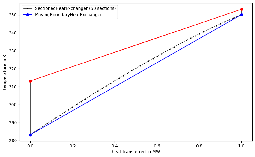
../_images/fc13b02002761029d40a5e873c944e3506a7574772bad877dab2c0555f0e4c68.png

Comparing the two again in a different situation: we preheat the working fluid with a relatively high pressure drop towards saturation. The difference shows on the secondary side (blue line).

def make_network_preheating(heatex):

    nw = Network()
    nw.units.set_defaults(
        temperature="°C",
        pressure="bar",
        pressure_difference="bar",
        heat="MW",
        heat_transfer_coefficient="kW/K"
    )
    so1 = Source("source 1")
    so2 = Source("source 2")
    si1 = Sink("sink 1")
    si2 = Sink("sink 2")
    c1 = Connection(so1, "out1", heatex, "in1", label="c1")
    c2 = Connection(heatex, "out1", si1, "in1", label="c2")
    d1 = Connection(so2, "out1", heatex, "in2", label="d1")
    d2 = Connection(heatex, "out2", si2, "in1", label="d2")
    nw.add_conns(c1, c2, d1, d2)
    c1.set_attr(fluid={"water": 1}, p=1, T=80)
    c2.set_attr(T=40)
    d1.set_attr(fluid={"R290": 1}, T=10, m=5)
    d2.set_attr(T_bubble=78, td_bubble=1)
    heatex.set_attr(dp1=0, dp2=4)
    return nw, c1, c2, d1, d2


hx_sectioned = SectionedHeatExchanger("heatexchanger")
nw_sectioned, c1, c2, d1, d2 = make_network_preheating(hx_sectioned)
nw_sectioned.solve("design")
heat_sect, T_hot_sect, T_cold_sect, _, _ = hx_sectioned.calc_sections()
heat_sect /= 1e6

hx_mb = MovingBoundaryHeatExchanger("heatexchanger")
nw_mb, c1, c2, d1, d2 = make_network_preheating(hx_mb)
nw_mb.solve("design")
heat_mb, T_hot_mb, T_cold_mb, _, _ = hx_mb.calc_sections()
heat_mb /= 1e6

fig, ax = plt.subplots(1, figsize=(10, 6))
ax.plot((heat_mb, heat_mb), (list(T_hot_mb), list(T_cold_mb)), color=annotation_color, linestyle="-", linewidth=0.5)
ax.plot(heat_sect, T_cold_sect, "o-", color=annotation_color, markersize=2, linewidth=0.5, label="SectionedHeatExchanger (50 sections)")
ax.plot(heat_mb, T_hot_mb, "o-", color="red")
ax.plot(heat_mb, T_cold_mb, "o-", color="blue", label="MovingBoundaryHeatExchanger")
ax.set_ylabel("temperature in K")
ax.set_xlabel("heat transferred in MW")
ax.legend()
plt.show()

 iter  | residual   | progress   | massflow   | pressure   | enthalpy   | fluid      | component  
-------+------------+------------+------------+------------+------------+------------+------------
 1     | 7.82e+05   | 1 %        | 4.67e+00   | 0.00e+00   | 0.00e+00   | 0.00e+00   | 0.00e+00   
 2     | 8.73e-07   | 100 %      | 5.21e-12   | 0.00e+00   | 0.00e+00   | 0.00e+00   | 0.00e+00   
 3     | 1.16e-10   | 100 %      | 6.95e-16   | 0.00e+00   | 0.00e+00   | 0.00e+00   | 0.00e+00   
 4     | 1.16e-10   | 100 %      | 6.95e-16   | 0.00e+00   | 0.00e+00   | 0.00e+00   | 0.00e+00   
Total iterations: 4, Calculation time: 0.00 s, Iterations per second: 2128.82

 iter  | residual   | progress   | massflow   | pressure   | enthalpy   | fluid      | component  
-------+------------+------------+------------+------------+------------+------------+------------
 1     | 7.82e+05   | 1 %        | 4.67e+00   | 0.00e+00   | 0.00e+00   | 0.00e+00   | 0.00e+00   
 2     | 8.73e-07   | 100 %      | 5.21e-12   | 0.00e+00   | 0.00e+00   | 0.00e+00   | 0.00e+00   
 3     | 1.16e-10   | 100 %      | 6.95e-16   | 0.00e+00   | 0.00e+00   | 0.00e+00   | 0.00e+00   
 4     | 1.16e-10   | 100 %      | 6.95e-16   | 0.00e+00   | 0.00e+00   | 0.00e+00   | 0.00e+00   
Total iterations: 4, Calculation time: 0.00 s, Iterations per second: 2703.39

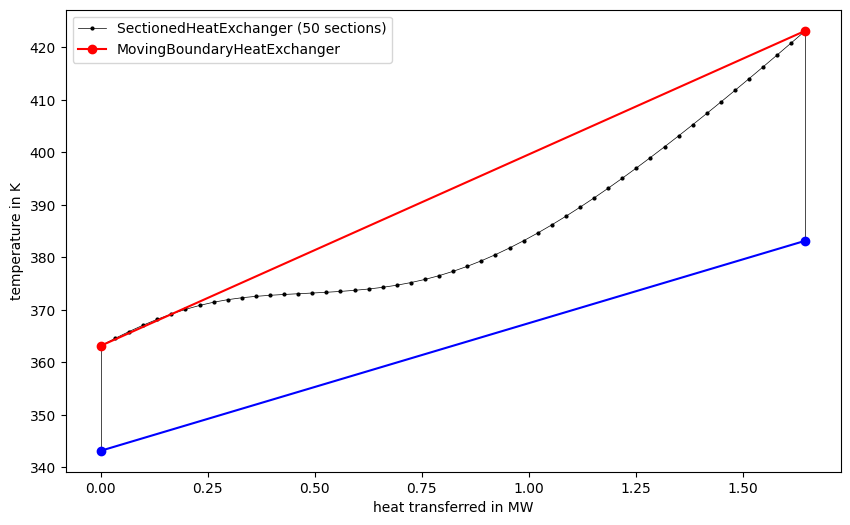
../_images/2019b3de0ad6a17ed9a755a91830276cd76b98c3d8a7a380f8024bfd5212141d.png

Curvature of isobars¶

Very similar to the previous comparison, in the supercritical region the sectioning is quite important.

def make_network_supercritical(heatex):

    nw = Network()
    nw.units.set_defaults(
        temperature="°C",
        pressure="bar",
        pressure_difference="bar",
        heat="MW",
        heat_transfer_coefficient="kW/K"
    )
    so1 = Source("source 1")
    so2 = Source("source 2")
    si1 = Sink("sink 1")
    si2 = Sink("sink 2")
    c1 = Connection(so1, "out1", heatex, "in1", label="c1")
    c2 = Connection(heatex, "out1", si1, "in1", label="c2")
    d1 = Connection(so2, "out1", heatex, "in2", label="d1")
    d2 = Connection(heatex, "out2", si2, "in1", label="d2")
    nw.add_conns(c1, c2, d1, d2)
    c1.set_attr(fluid={"R290": 1}, T=150, p=45, m=5)
    c2.set_attr(T=90)
    d1.set_attr(fluid={"water": 1}, p=2, T=70)
    d2.set_attr(T=110)
    heatex.set_attr(dp1=0, dp2=0)
    return nw, c1, c2, d1, d2


hx_sectioned = SectionedHeatExchanger("heatexchanger")
nw_sectioned, c1, c2, d1, d2 = make_network_supercritical(hx_sectioned)
nw_sectioned.solve("design")
heat_sect, T_hot_sect, T_cold_sect, _, _ = hx_sectioned.calc_sections()
heat_sect /= 1e6

hx_mb = MovingBoundaryHeatExchanger("heatexchanger")
nw_mb, c1, c2, d1, d2 = make_network_supercritical(hx_mb)
nw_mb.solve("design")
heat_mb, T_hot_mb, T_cold_mb, _, _ = hx_mb.calc_sections()
heat_mb /= 1e6
heatex = SectionedHeatExchanger("heatexchanger")

fig, ax = plt.subplots(1, figsize=(10, 6))
ax.plot((heat_mb, heat_mb), (list(T_hot_mb), list(T_cold_mb)), color=annotation_color, linestyle="-", linewidth=0.5)
ax.plot(heat_sect, T_hot_sect, "o-", color=annotation_color, markersize=2, linewidth=0.5, label="SectionedHeatExchanger (50 sections)")
ax.plot(heat_mb, T_hot_mb, "o-", color="red", label="MovingBoundaryHeatExchanger")
ax.plot(heat_mb, T_cold_mb, "o-", color="blue")
ax.set_ylabel("temperature in K")
ax.set_xlabel("heat transferred in MW")
ax.legend()
plt.show()

 iter  | residual   | progress   | massflow   | pressure   | enthalpy   | fluid      | component  
-------+------------+------------+------------+------------+------------+------------+------------
 1     | 1.39e+06   | 0 %        | 8.23e+00   | 0.00e+00   | 0.00e+00   | 0.00e+00   | 0.00e+00   
 2     | 2.64e-07   | 100 %      | 1.57e-12   | 0.00e+00   | 0.00e+00   | 0.00e+00   | 0.00e+00   
 3     | 2.33e-10   | 100 %      | 1.38e-15   | 0.00e+00   | 0.00e+00   | 0.00e+00   | 0.00e+00   
 4     | 2.33e-10   | 100 %      | 1.38e-15   | 0.00e+00   | 0.00e+00   | 0.00e+00   | 0.00e+00   
Total iterations: 4, Calculation time: 0.00 s, Iterations per second: 2161.18

 iter  | residual   | progress   | massflow   | pressure   | enthalpy   | fluid      | component  
-------+------------+------------+------------+------------+------------+------------+------------
 1     | 1.39e+06   | 0 %        | 8.23e+00   | 0.00e+00   | 0.00e+00   | 0.00e+00   | 0.00e+00   
 2     | 2.64e-07   | 100 %      | 1.57e-12   | 0.00e+00   | 0.00e+00   | 0.00e+00   | 0.00e+00   
 3     | 2.33e-10   | 100 %      | 1.38e-15   | 0.00e+00   | 0.00e+00   | 0.00e+00   | 0.00e+00   
 4     | 2.33e-10   | 100 %      | 1.38e-15   | 0.00e+00   | 0.00e+00   | 0.00e+00   | 0.00e+00   
Total iterations: 4, Calculation time: 0.00 s, Iterations per second: 2827.78

../_images/ae04f22821eba66c9dd5ea87c19f24e6c5d02723dd91dc80d1241307904297f8.png